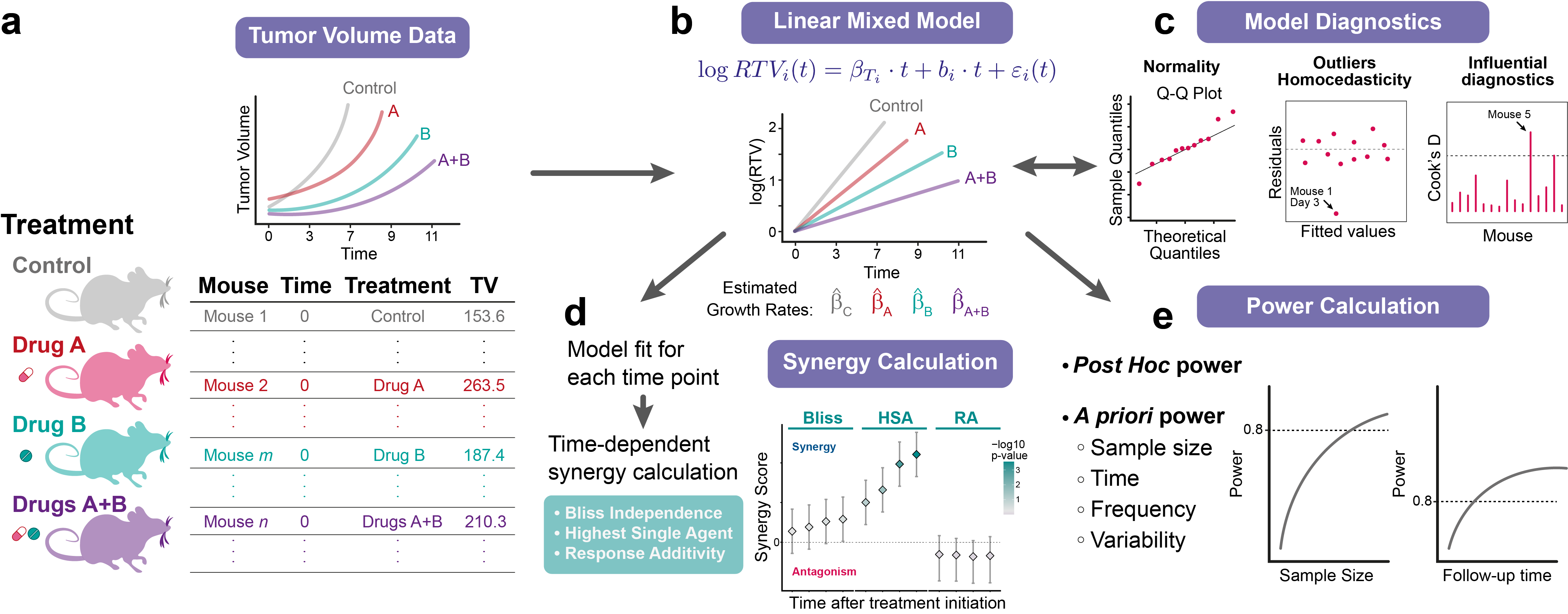
SynergyLMM Workflow Overview
How to Use SynergyLMM
Welcome to the SynergyLMM tutorial!
This quick-start tutorial shows how to use the web-app.
An example dataset will be used,
which can be downloaded by clicking in the link below:
Data Upload and Model Fit
The user can upload the data in the 'Model Estimation' tab. The input data should be a data table in long format with at least four columns: one for sample IDs, one for time points, one for treatment groups, and one for tumor volume measurements. (See the example dataset for reference).
This is how the data should look like:
Input Table
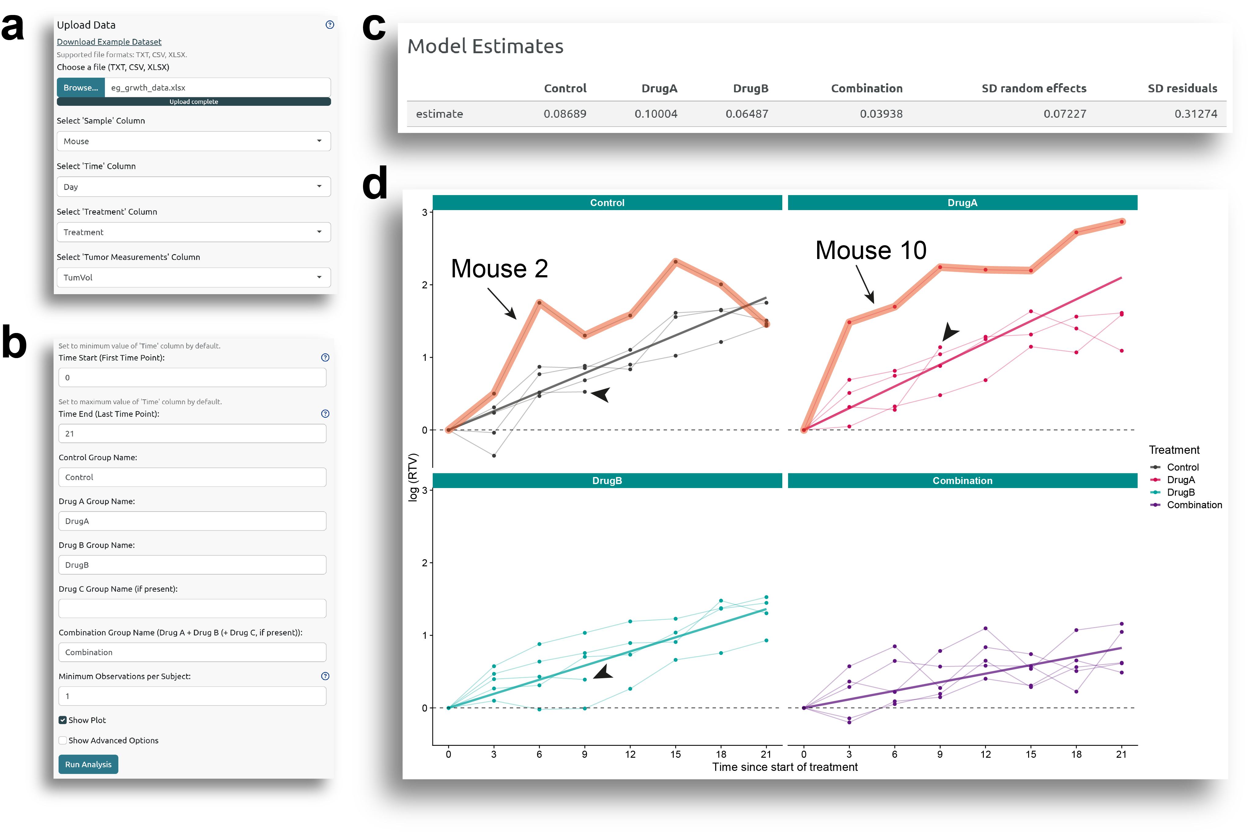
Once the data is uploaded, the user will need to specify which columns contain each information. For this example, columns Mouse, Day, Group, and TumVol contain the information about the sample IDs, time points, treatments, and tumor measurements, respectively (Fig. 1a).
The next step is to define the time points for the experiment. By default, the minimum and maximum values in the 'Time' column will be used as the start and end time points, but these can be modified. The name of the different treatments in the experiment also need to be specified. In this example, 'Control', 'DrugA', 'DrugB', and 'Combination' correspond to the control, single drugs, and the drug combination groups (Fig. 1b).
Next, clicking on 'Run Analysis' will fit the model and produce a table with the model estimates, (Fig. 1c), including the tumor growth rates of the different groups, and the standard deviations for the random effects and for the residuals. If 'Show Plot' is selected, the plots with the tumor growth curves are displayed along with the regression line for the fixed effect coefficients (i.e., the tumor growth rates for the control and treatment groups, Fig. 1d).
The orange-shaded lines in Fig. 1d indicate two individuals, mouse 2 and mouse 10, whose measurements are (intentionally) notably different from the others, and which will greatly affect the model and the results. The impact of these individuals and how to deal with them will be discussed later.
Minimum Observations per Subject and Growth Model
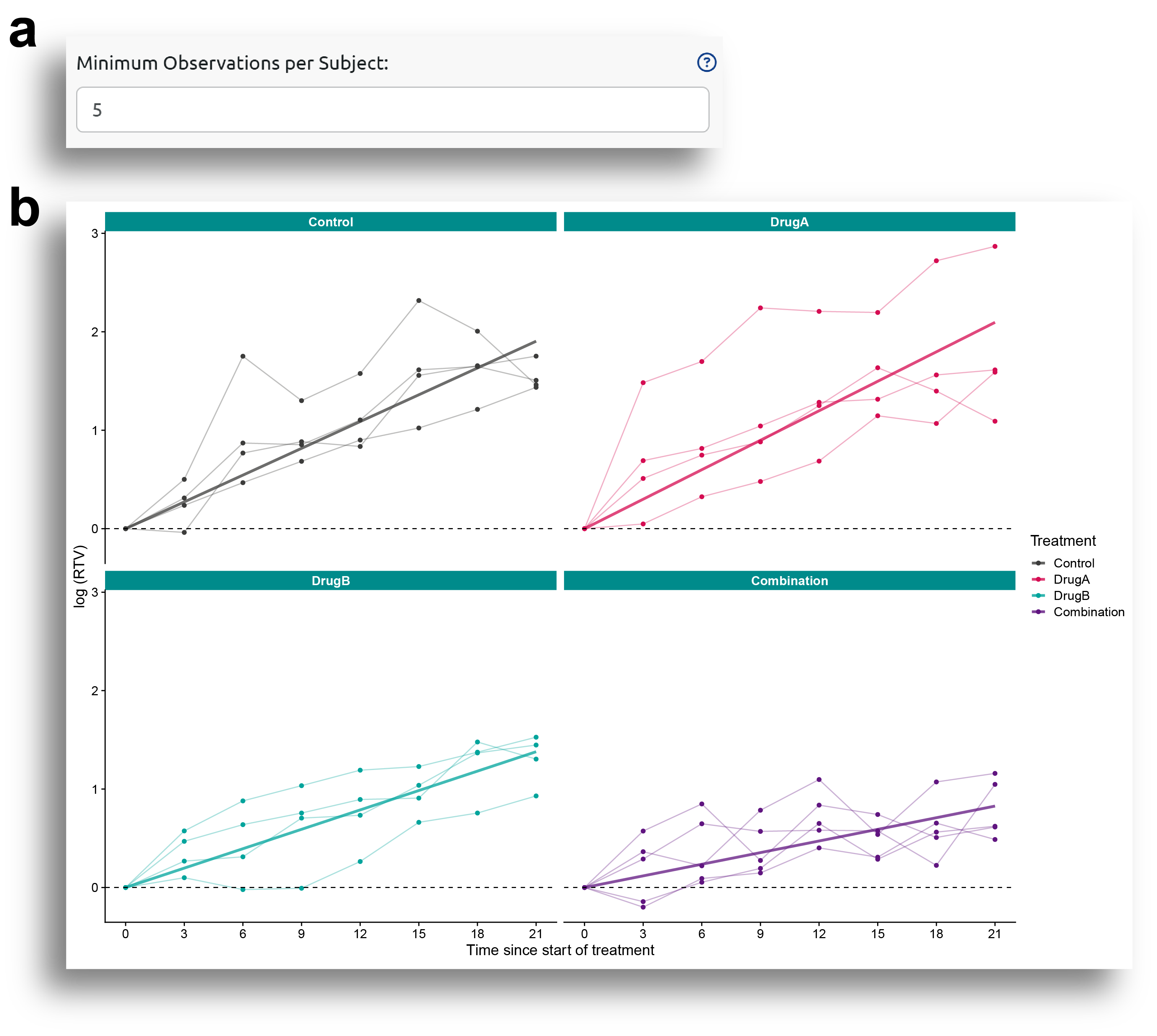
In Fig. 1b, there is an option called
'Minimum Observations per Subject'
, which allows for excluding
samples with fewer than the specified number of observations. For example, in Figure 1d, the arrow heads indicate
subjects for which only four observations were made. If the the minimum observations per subject is set to five,
these samples will be omitted from the analysis (Fig 2).
Fig. 1b also shows an option called
'Growth Model'
. This box allows to choose between 'Exponential' or 'Gompertz' growth models. The exponential
model is fitted using a linear mixed effect model, while the Gompertz model is fitted using a non-linear mixed effect model.
The exponential model is generally a good starting point for most in vivo studies, and it tends to converge more easily. However, it may be
insufficient when tumor growth dynamics deviate significantly from exponential behavior. In such cases, the Gompertz model typically
offers better flexibility and more accurate estimates of tumor growth and treatment effects.
Synergy Analysis
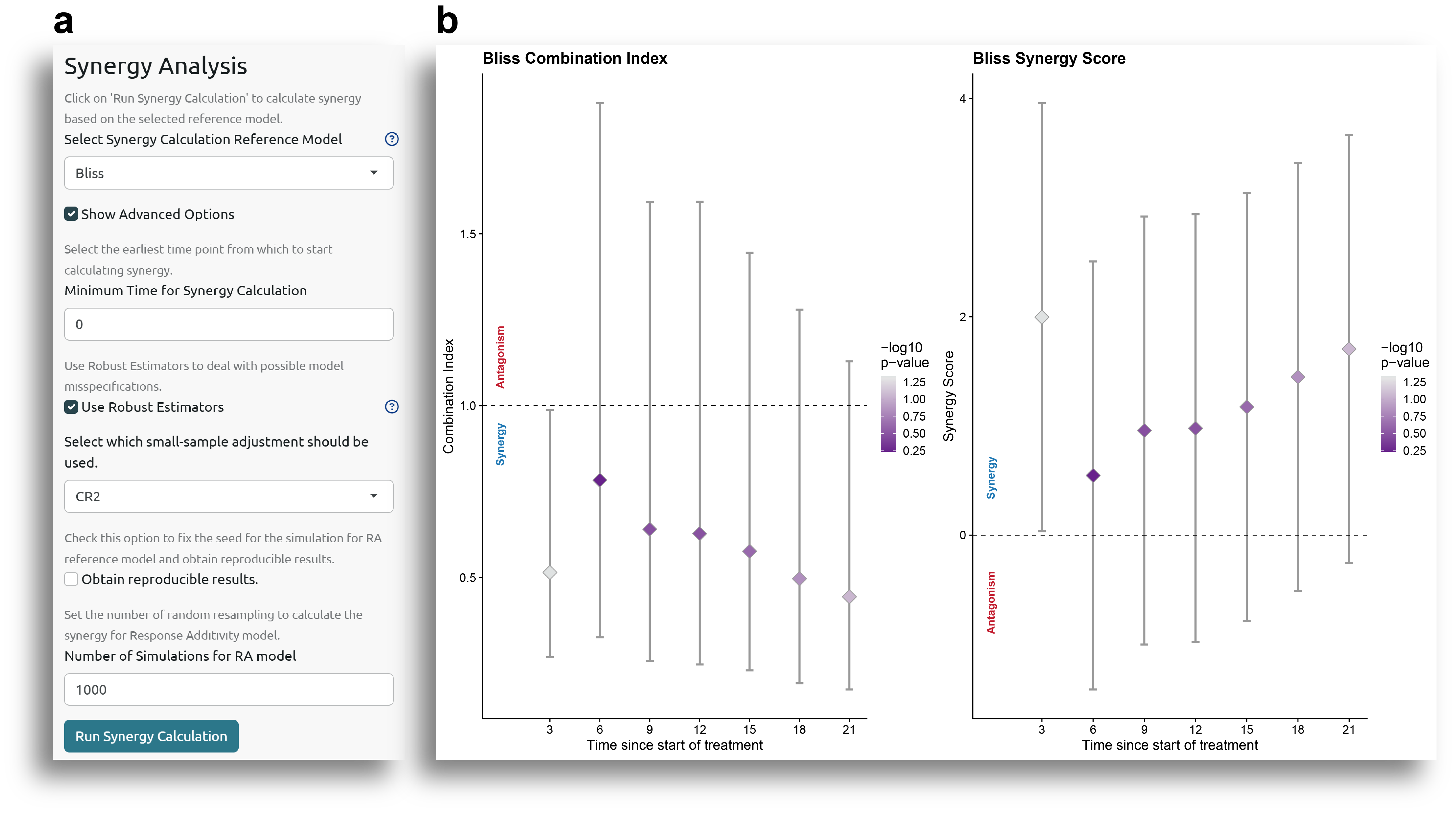
Once the model is fitted, the Synergy Analysis can be performed. Fig. 3a shows the different options for synergy analysis. The user can choose between Bliss, highest single agent (HSA), or response additivity (RA) reference models. In the advance options, selecting 'Use Robust Estimators' will apply sandwich-based cluster-robust variance estimators. This is recommended and can help to deal with possible model misspecifications.
The analysis for the response additivity reference model is based on simulations, and the number of simulations to run can also be specified by the user.
Fig. 3a also shows two additional options for the statistical assessment of synergy, 'Confidence level' and 'Correction method for adjusting p-values'. The first one allows the user to choose the confidence level for the confidence intervals and p-values calculation (default to 0.95), while the second one allows the user to choose between different methods for multiple comparison synergy p-values adjustment. More information about the available methods can be obtained by clicking in the '?' help menu.
The output of the analysis includes a plot with the combination index (CI) and synergy score (SS) for each time point (Fig. 3b), as well as a table with all the results. The plot in Fig. 3b shows the estimated synergy metric (CI or SS) value, together with the confidence interval (vertical lines), and the color of the dots indicates the statistical significance.
The interpretation of the CI and SS values follows the typical definition of CI and SS:
- CI: Provides information about the observed drug combination effect versus the expected additive effect according to the reference synergy model. A drug combination effect larger than the expected (CI > 1) indicates synergism, a drug combination effect equal to the expected (CI =1) indicates additivity, and a lower drug combination effect than the expected (CI < 1) indicates antagonism. The value of the CI represents the proportion of tumor cell survival in the drug combination group compared to the expected tumor cell survival according to the reference model.
- SS: The synergy score is defined as the excess response due to drug interaction compared to the reference model. Following this definition, a SS>0, SS=0, and SS<0, represent synergistic, additive and antagonistic effects, respectively.
Synergy Results
As observed in Fig. 3b and the table with the results, the only time point for which there is a statistically significant
result is time 3. At this time point, the CI is lower than 1, and the SS is higher than 0, indicating
synergy in the drug combination group. However, at the other time points, the results show that the confidence
interval includes 1 for the CI and 0 for the SS, and the p-value is higher than 0.05, indicating that
the additive effect of the drug combination cannot be rejected.
In addition to the synergy results, a table output with the model estimates is also returned. In the case of using the exponential model,
as a model is fitted for each time window being analyzed, the model estimates for each time point are reported:
Model Estimates by Time
Model Diagnostics
An important step in the analysis is to verify that the model is appropriate for the input data. In the Model Diagnostics tab, the user can check the main assumptions: the normality of the random effects and the residuals.
The model diagnostics output includes four plots to help evaluate the adequacy of the model. The two plots at the top of Fig. 4a show the Q-Q plot of the random effects and normalized residuals. Most points in these plots should fall along the diagonal line. The two plots at the bottom of Fig. 4a show scatter plots of the standardized residuals versus fitted values and standardized residuals per time and per treatment, which give information about variability of the residuals and possible outlier observations. The residuals in these plots should appear randomly distributed around the horizontal line, indicating homoscedasticity. Fig. 4b shows the output of Shapiro-Wilk normality tests for the random effects and the residuals. A non-significant p-value obtained by the Shapiro-Wilk normality indicates that there is no evidence to reject normalilty.
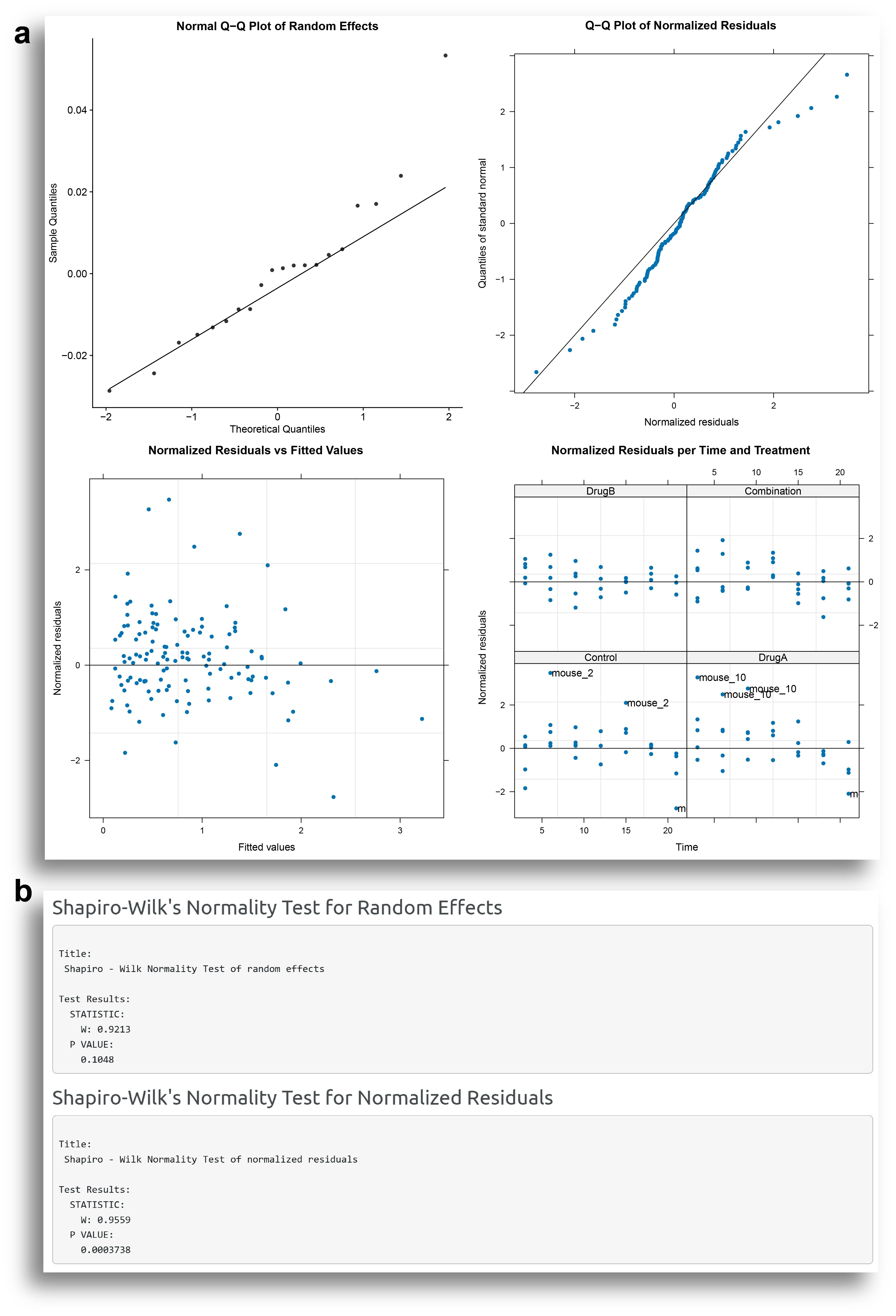
The results from the plots and the normality tests seem to indicate some departure from the normality, especially evident for the residuals. This could be related to those individuals which has a large variation in the measurements.
Observations with absolute normalilzed residuals greater than the 1−0.05/2 quantile of the standard normal distribution are identified as potential outlier observations. A table with these observations is also provided by SynergyLMM. It can be observed that many observations from mouse 2 and mouse 10 have large residual values.
Potential Outlier Observations
As mentioned before, mouse 2 and mouse 10 are intentionally introduced outliers in the model, and there are many observations from these subjectes that are indeed identified as potential outliers. More details about outlier identification are provided in the Influential Diagnostics section. But first, there are several approaches that the user can follow to try to improve the model diagnostics.
If the diagnostic plots and tests show evident violations of the model assumptions, there are several solutions that may help improving the model:
-
- Transform the time variable:
Both exponential and Gompertz models are based on ordinary differential equations (ODEs),
which can be formulated using arbitrary time scales. Applying transformations, such as the square root or logarithm (with +1 offset),
can often improve model fit, enhance linearity, stabilize variance, and ensure better numerical performance. Importantly, when comparing
the exact values of a drug combination synergy index, the models should use the same timescale
-
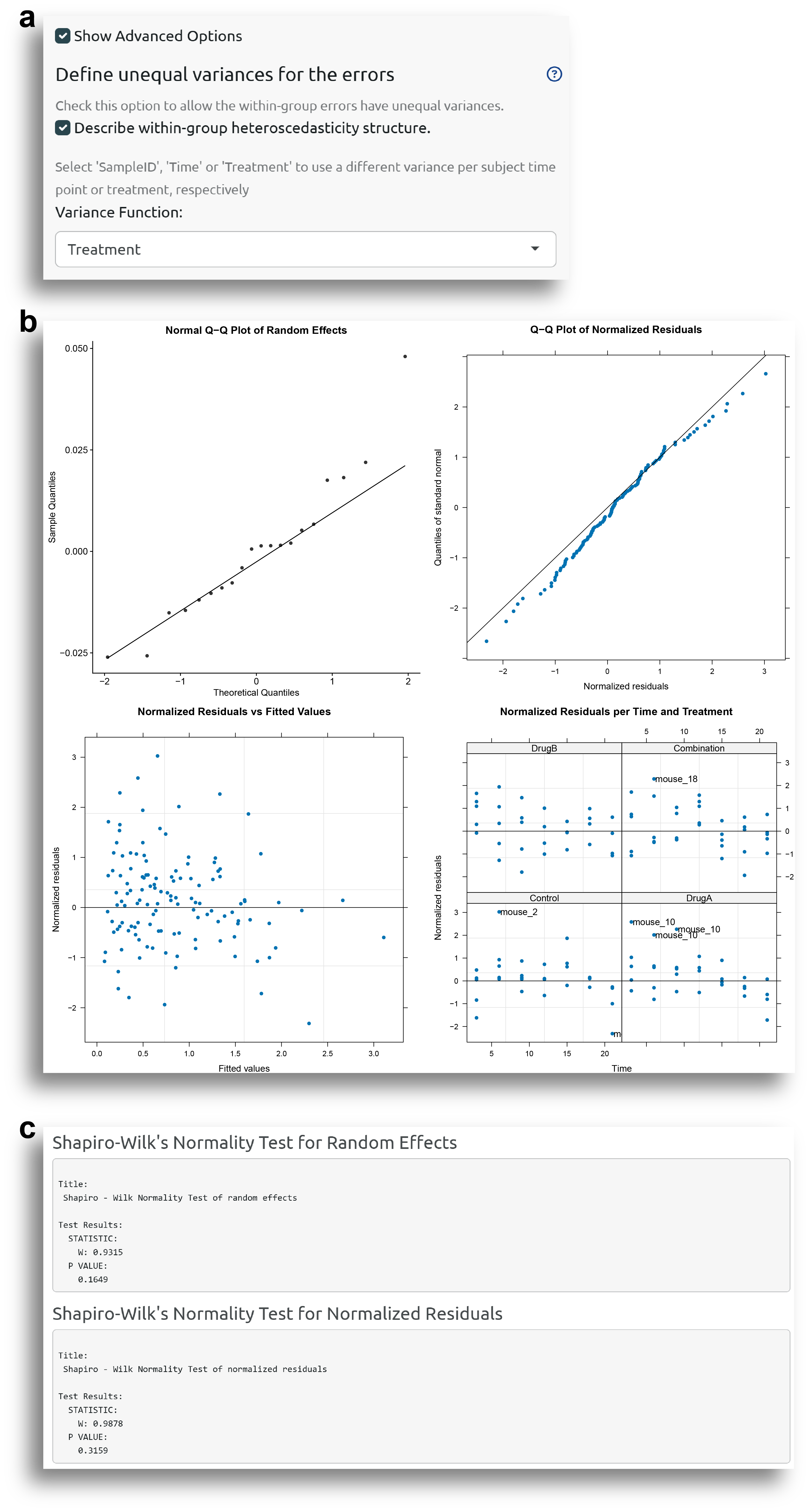
- Specify a residual variance structure:
SynergyLMM uses the ‘nlme’ R package, which supports flexible variance and correlation structures.
These allow for heterogeneous variances or within-group correlations, such as those based on subject, time point, treatment, or combinations of these.
Applying these structures can substantially improve model diagnostics and the robustness of the estimates. This can be done in the
Advanced Options
of the
Model Estimation
tab.
-
- Prefer the Gompertz model when the exponential model fails:
While the exponential model is generally a good starting point for most
in vivo studies, and it tends to converge more easily, it may be insufficient when tumor growth dynamics deviate significantly from exponential
behavior. In such cases, the Gompertz model typically offers better flexibility and more accurate estimates of tumor growth and treatment effects.
-
- Carefully address potential outlier:
Individuals or measurements highlited as potential outliers may warrant
further investigation to reveal the reasons behind unusual growth behaviours, and potentially exclude these before re-analysis,
after careful reporting and justification.
In this case, the model will be fitted especifying a unequal variance for the errors. Concretely, a different variance for each treatment is defined (Fig. 5a). It can be seen that this has improved the model diagnostics, and now both the random effects and normalized residuals are approximately normally distributed. There are still some potential outlier observations, which is normal, since there are two intentional outlier subjects.
Influential Diagnostics
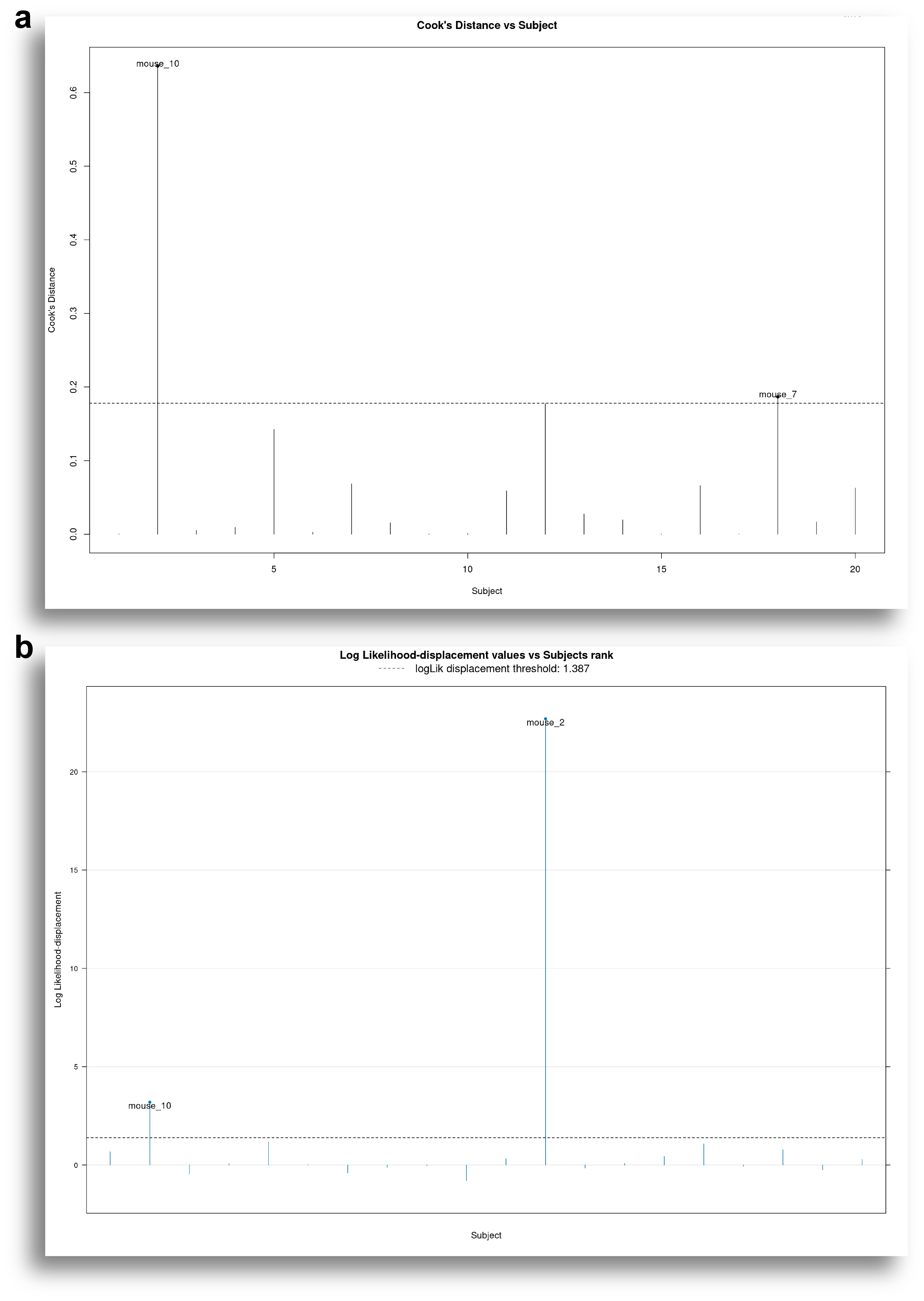
The Influential Diagnostics tab is useful to identify subjects that have a great impact in the model and that may warrant more careful analysis. To this end, SynergyLMM uses subject-specific Cook's distances.
Cook's distances can be calculated based on the change in fitted values, or based on the change in the fixed effects.
Cook's distances based on the change in fitted values assess the influence of each subject on the model fit. On the other hand, Cook's distance based on the change in fixed effect values assess the influence of each subject in the estimated parameters of the treatment groups.
Fig. 6 shows results of the influential diagnostics of our example model. It can be seen how Mouse 10 is identified as having a great influence in the fitted values.
Model Performance
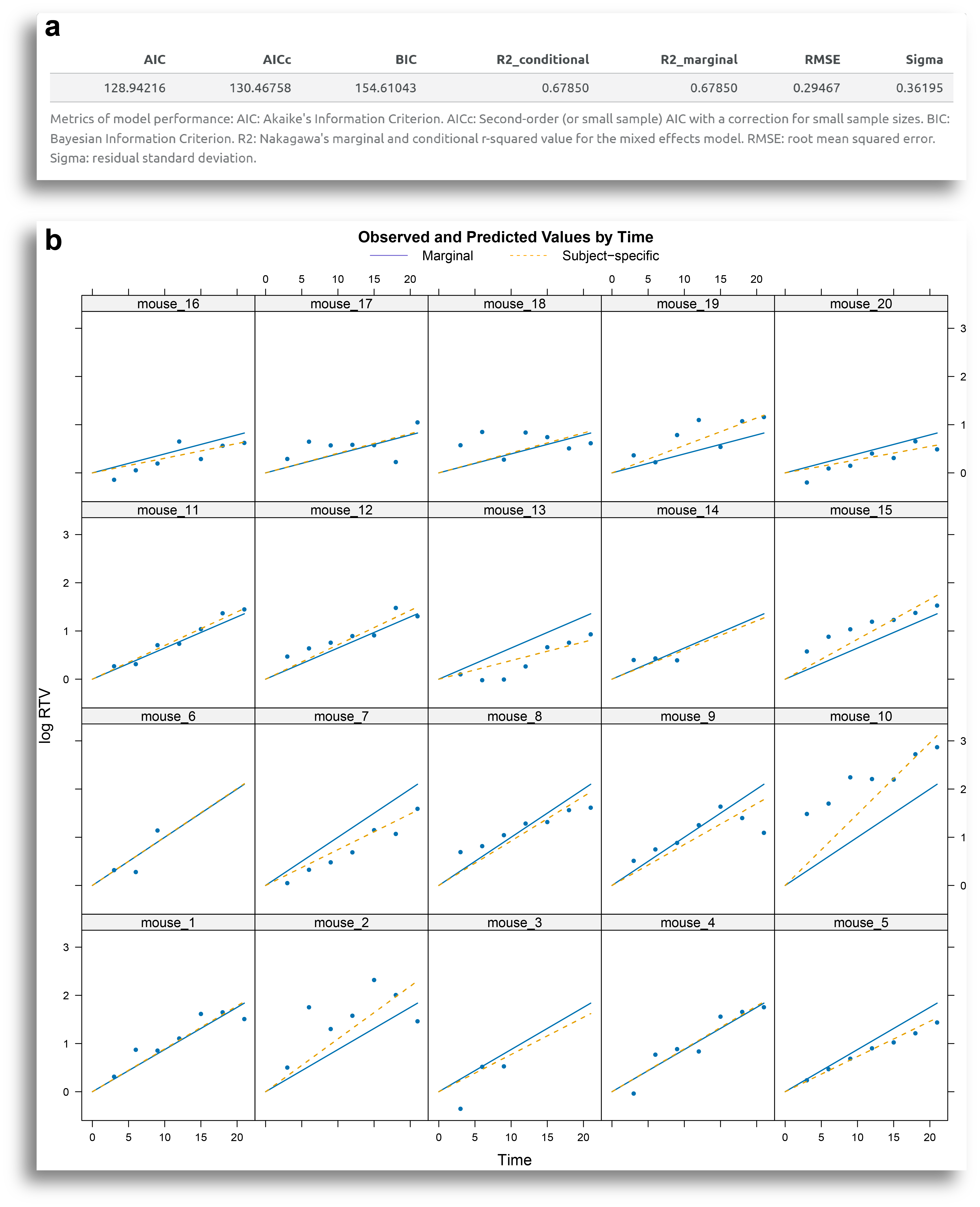
Another important tool for the diagnostics of the model is the plot of the observed vs. predicted values, available in the Model Performance tab. The output from this tab includes a table with model performance metrics, such as R-square and various error measures (Fig. 7a), along with the plot of observed vs. predicted values (Fig. 7b).
Each plot in Fig. 7b corresponds to a subject. The blue dots represent the actual measurements, the continuous line shows the group (treatment) marginal predicted values, and the dashed line indicates each individual's predicted values
By examining how closely the lines fit the data points, the user can assess how well the model fits the data. In this example, the model generally fits the data well, except for certain subjects, such as mouse 2 and mouse 10.
Power Analysis
Note: Power analyses are only available for models fitted using the exponential growth model.
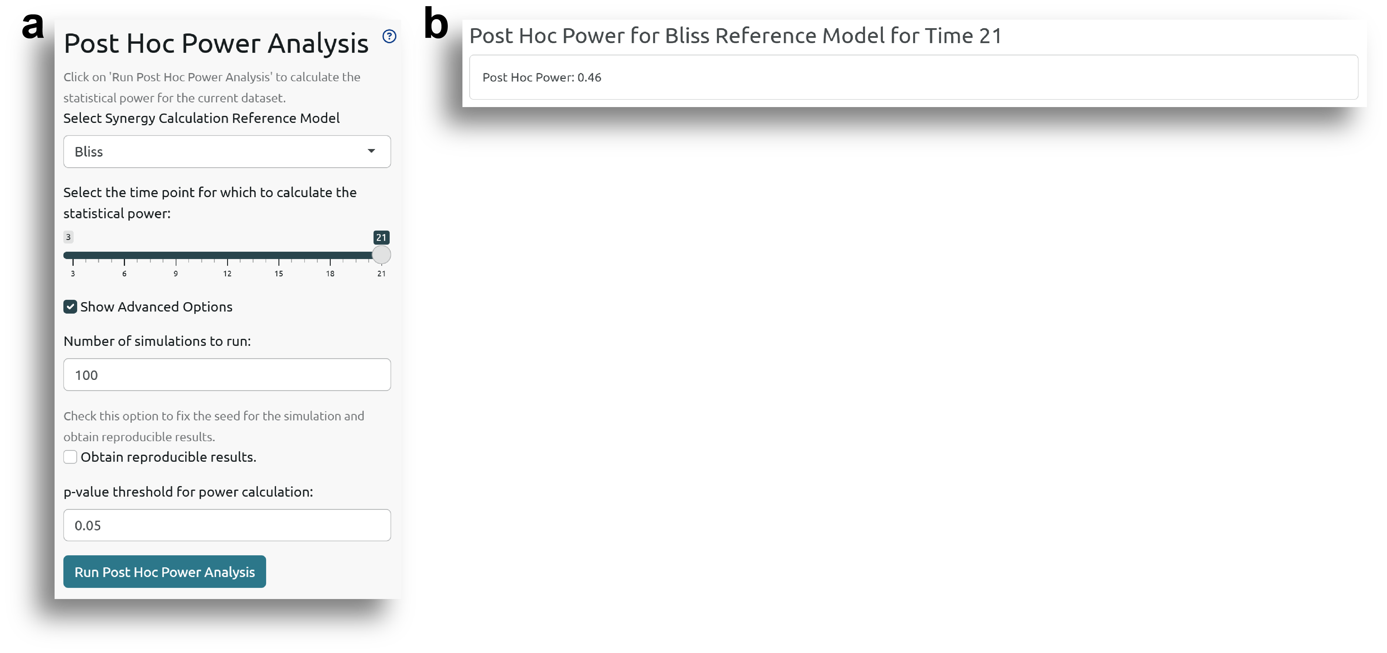
Post Hoc Power Analysis
The Post Hoc Power Analysis allows users to check the statistical power of the dataset and fitted model for synergy analysis using the Bliss and HSA reference models.
The post hoc power calculation is based on simulations, and depending on the dataset, it can take some time to run. The power is returned as the proportion of simulations resulting in a significant synergy hypothesis test.
Fig. 8a shows the side panel for running the post hoc power analysis. The user can define the number of simulations to run, the p-value threshold for considering significance, and the time point for which to perform the analysis.
A Priori Power Analysis
The user can also perform three different types of a priori power analyses by modifying various experimental variables. To do this, 'SynergyLMM' creates exemplary datasets using the estimates from the fitted model in the Model Estimation tab. Then, several parameters can be modified and evaluated by the user, such as: the number of subjects per group, the days of measurements, the coefficients (tumor growth rates) for each treatment group, the standard deviation of the random effects (between-subject variance), and the standard deviation of the residuals (within-subject variance).
SynergyLMM then provides the a priori power calculation for each exemplary dataset defined by a specific set of experimental parameters.
Sample Size
The first option that can be tested is how the power would vary as the sample size per group changes. To do this, an exemplary dataset is used to fit models with the same values for all parameters (coefficients for the different treatment groups, standard deviations of the random effects and residuals, number of time points, etc.) as in the fitted model, but varying the sample size in each group. The user can select the range of sample sizes to evaluate and the reference model to use (Fig. 9a).
When clicking 'Run Sample Size Power Analysis', a plot with the exemplary data and another showing the power variation with the sample size are displayed (Fig. 9b). It can be confirmed that the values shown in the exemplary data plot are the same as the model estimates shown in Fig. 1c.
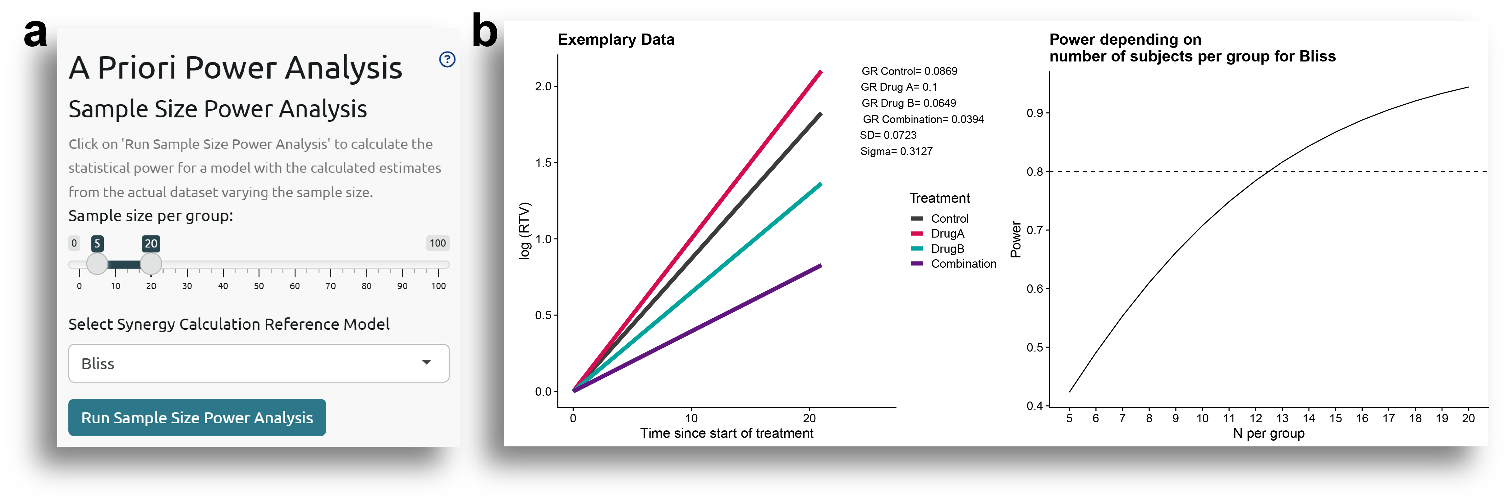
The results from the a priori power analysis show that to achieve a statistical power of 0.8, and assuming the other parameters remain constant, the sample size per group should be at least 13.
Time Power Analysis
Another parameter that can affect statistical power is the duration of follow-up or the frequency of measurements. Given the results of a pilot experiment, the user may wonder how the results would change if tumor growth were monitored for a longer time period, or how often tumor growth measurements should be taken. To address this, the user can evaluate statistical power by varying the maximum follow-up time or the frequency of measurements, while keeping the other parameters fixed, as determined from the fitted model.
Maximum Time of Follow-up
First, it can be examined how power changes if the follow-up time is increased or decreased. To do this, select the analysis based on the maximum time of follow-up ('max'), as shown in Fig. 10a. The sample size per group, the time interval between measurements, and the reference model to use can be also specified. For this example, the analysis evaluated how power varied from 3 to 42 days of follow-up, with 5 subjects per group, and measurements taken every 3 days.
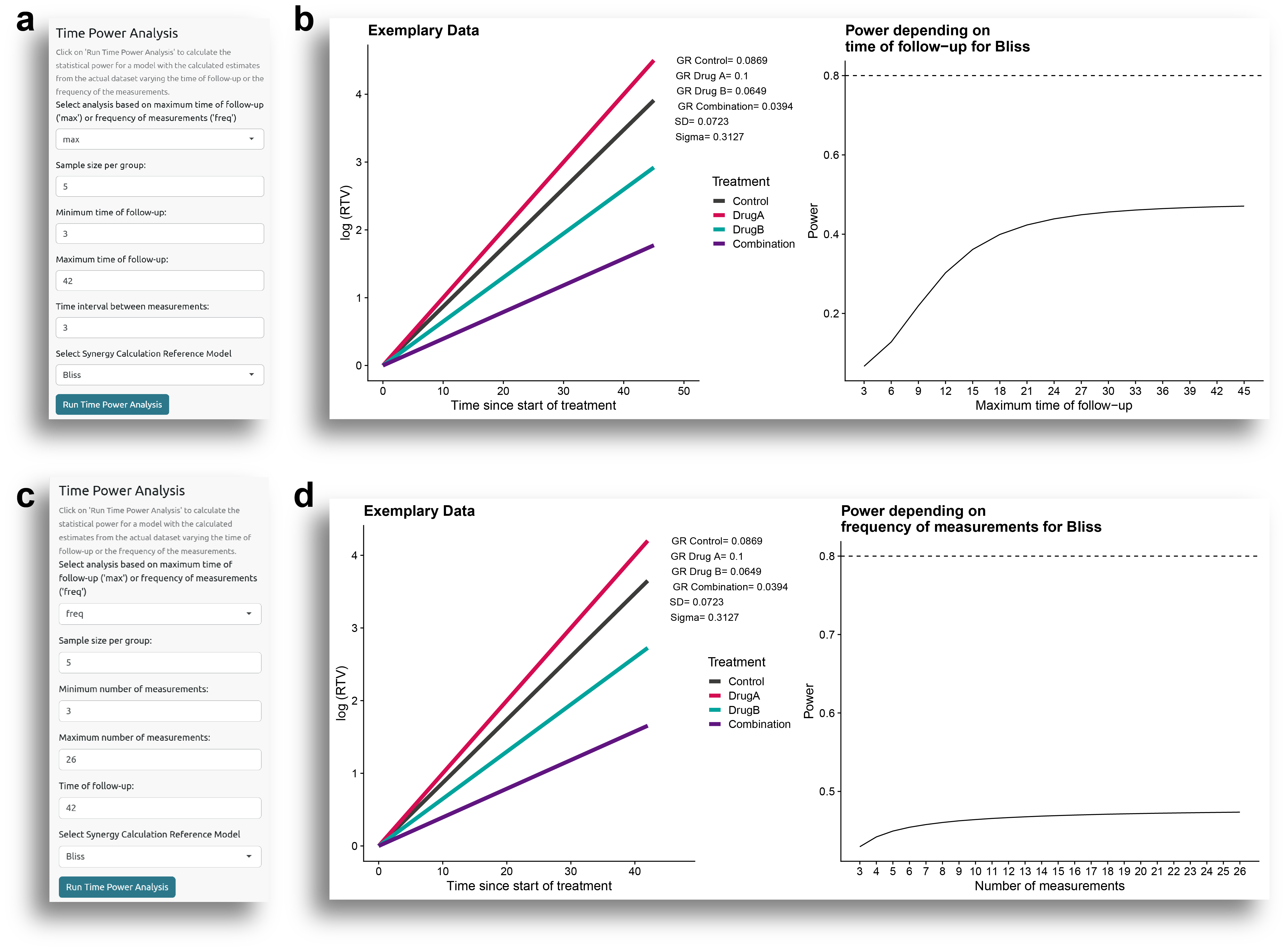
In Fig. 10b, it can be seen how the power varies with the maximum time of follow-up. As expected, when the follow-up period is short, the statistical power is low, and it increases as the follow-up time increases, until it reaches a point where the power does not increase significantly.
Frequency of Measurements
Another question that researchers may have is how frequently the measurements should be taken. Of course, this would depend, among other factors, on practical considerations, but it can be simulated to estimate the ideal frequency of measurements.
Again, for this analysis, all the parameters are fixed, and the only variation is how frequently the measurements are taken, which is defined by the number of evenly spaced measurements performed during the follow-up period. For this example, the analysis evaluated how the power varied from 3 to 26 evenly spaced measurements, with 5 subjects per group and a follow-up period of 42 days (Fig. 10c).
As shown in Fig. 10d, the power increases as the number of measurements increases, although the difference is not dramatic.
Data Variability Power Analysis
Finally, another factor that can affect statistical power is the variability in the data. The variability in the model is represented by the standard deviation of the random effects (between-subject variability) and the standard deviation of the residuals (within-subject variability), which can be obtained from the table shown in Fig. 1c.
Additionally, the statistical power is also influenced by the magnitude of the differences: the greater the effect of the drug combination, the higher the statistical power to detect synergistic effects.
The user can test how statistical power varies by modifying the variability and the drug combination effects in the 'Variability Power Analysis' side panel (Fig. 11a).
In this case, the parameters that vary are the standard deviations of the random effects and the residuals, as well as the effect of the drug combination, represented by the coefficient of the drug combination group (i.e., tumor growth rate in the drug combination group). By default, these parameters are evaluated over a range from 10% to 200% of the values obtained from the model fitted in the Model Estimation tab, but they can be modified by checking the 'Show Advanced Options' box.
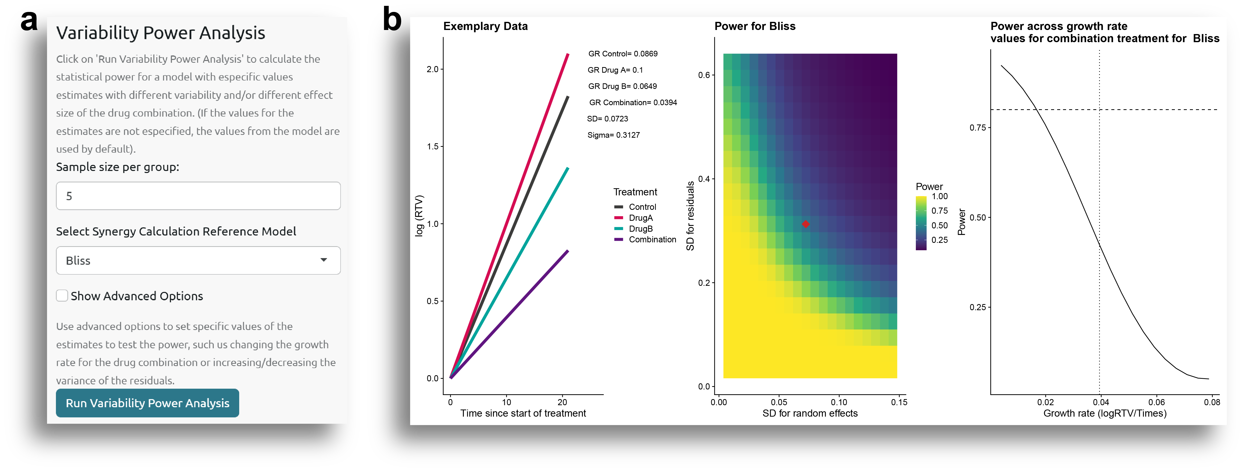
From the results shown in Fig. 11b, it can be observed how the power increases as the variability decreases and as the coefficient for the drug combination group decreases (i.e., the growth rate for the drug combination is smaller, indicating a higher drug combination effect).
Recommended workflow for using SynergyLMM
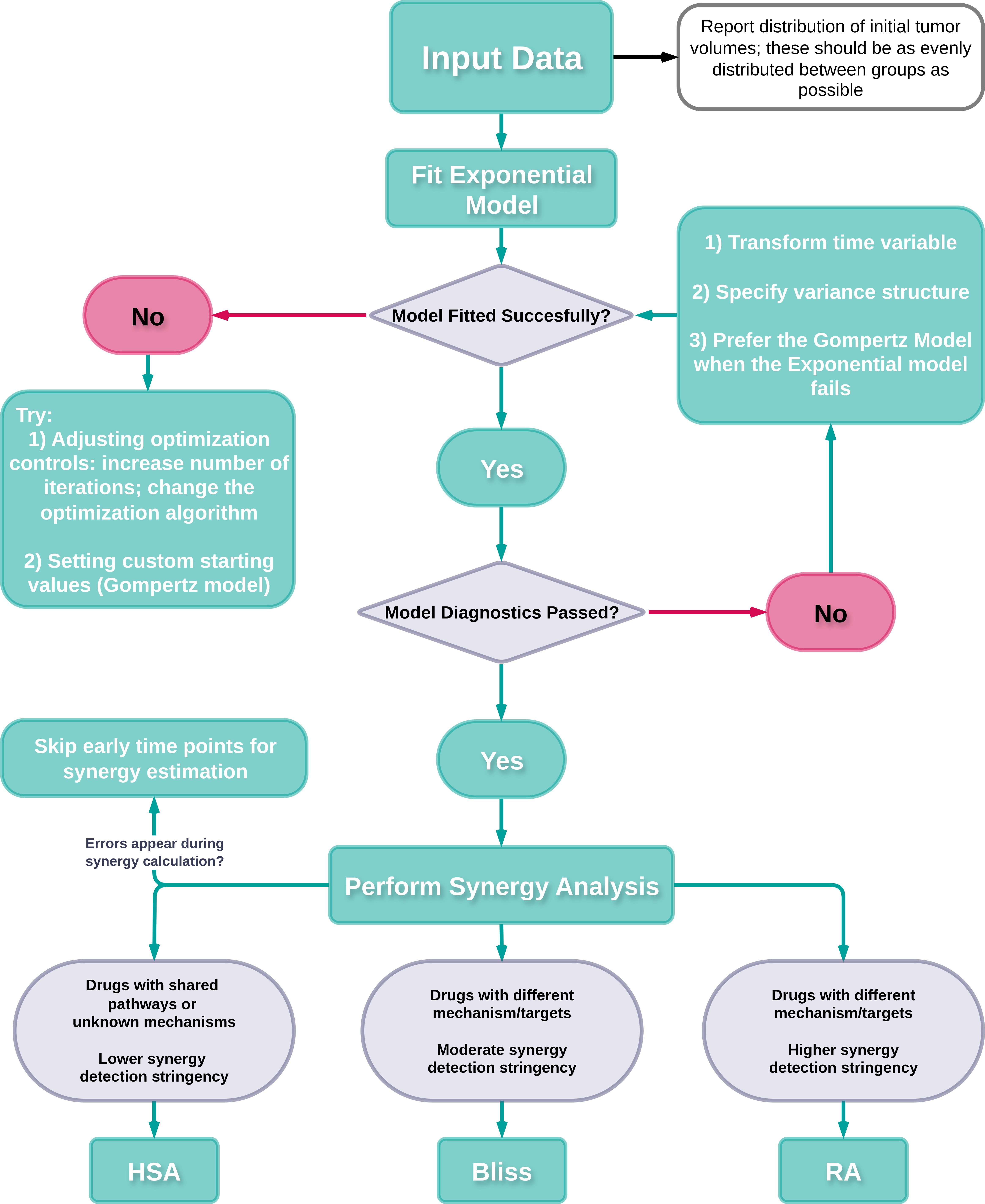
Recommended workflow for using SynergyLMM to assess drug combination effects. HSA: highest single agent. RA: response additivity.